Phylogenetics: R Primer

	EEB 349: Phylogenetics
	This lab represents an introduction to the R computing language, which will be useful for upcoming homework assignments as well as for software written as R extensions (i.e. APE)

What is R?

R is one of two programming languages that we will use this semester (the other being Python). One might make the case that programs like PAUP that are associated with a unique command language also represent programming languages; however, R and Python are different in being general purpose (i.e. not written specifically for phylogenetics).

While R and Python share many similarities, R excels in tasks that involve statistics and creating plots. While a spreadsheet program like Excel can create charts, it is often easier to create the plot you need in R. The purpose of this lab is to introduce you to R by showing you how to make various plots related to probability distributions. This will also enable you to learn about several important probability distributions that serve as prior distributions in Bayesian phylogenetics.

Installing R

Install the R package by going to http://www.r-project.org/ and following the download instructions for your platform.

Some R basics

To use R, type commands into the console window at the R prompt (>). Try these commands for starters:

> help()
> help(plot)
> help.search("gamma")

Creating a plot

Let's begin by making a simple scatterplot using these data:

x	y
1	1
2	1
1	3
4	5
2	4
3	5
4	7
5	8

In the R console window, enter the data and plot it as follows (note that you should not type the initial > on each line; that's the R prompt):

> x <- c(1,2,1,4,2,3,4,5)
> y <- c(1,1,3,5,4,5,7,8)
> plot(x,y)

The left-pointing arrow is the assignment operator: x <- y means assign y to x. The c(...) notation is carried over from its progenitor, the S language. The "c" means "column" and is derived from the fact that mathematical vectors are columns of a matrix (and the c(...) notation is used to input a vector). All we need be concerned about is that a vector of values should be input as a comma-delimited list surrounded by parentheses and preceded by the letter "c".

Modifying a plot

R does a fairly nice job of selecting defaults for plots, but I find myself wanting to tweak things. This section explains how to modify various aspects of plots.

Changing the plotting symbol

Use the pch parameter to change the symbol R uses to plot points:

> plot(x, y, pch=19)

Common values for pch include 19 (solid dot), 20 (bullet), 21 (circle), 22 (square), 23 (diamond), 24 (up-pointing triangle), and 25 (down-pointing triangle). The stroke and fill color for symbols 21-25 can be changed using the col and bg parameters. For example, to use red squares with yellow fill, try this:

> plot(x, y, pch=22, col="red", bg="yellow")

Search for the help topic on points for more info:

> help.search(points)

Plot type

The default plot type is "p" for points, but other plot types can be used (use the command help(plot) for details). Let's use the "l" (that's a lower-case L) type to connect our points with lines:

> plot(x, y, type="l")

Clearly, this is not something that you would want to do with these data, but we will use type="l" extensively later in this tutorial. To use both points and lines, set the type to both ("b"):

> plot(x, y, type="b")

Line width

To make the line connecting the points thicker, use the lwd option (lwd=1 is the default line width):

> plot(x,y,type="l",lwd=3)

Plot and axis labels

The xlab, ylab and main parameters can be used to change the x-axis label, the y-axis label and the main plot title, respectively:

> plot(x, y, type="l", xlab="width", ylab="height", main="Leaf width vs. height")

Losing the box

The bty parameter can be set to "n" to remove the box around the plot:

> plot(x, y, type="l", bty="n")

Losing an axis

The xaxt and yaxt parameters can be set to "n" to remove the x- and y-axis, respectively, from the plot. Here for example is a plot with no y-axis (note that I've also set the y-axis label to an empty string with ylab="" and removed the box around the plot with bty):

> plot(x, y, type="l", yaxt="n",ylab="",bty="n")

Changing axis labeling

It is often desirable to change the values used on the x- or y-axis. You can use the ylim parameter to make the y-axis extend from 0 to 10 (instead of the default, which is 1 to 8 in this case because that is the observed range of y values):

> plot(x, y, type="l", ylim=c(0,10))

Note that there is a little overhang at both ends on the y-axis (the 0 tick mark is slightly above the bottom of the plot and the tick mark for 10 is slightly below the top of the plot). This is because, by default, the y-axis style parameter yaxs is set to "r", which causes R to extend the range you defined (using ylim) by 4% at each end. You can set yaxs="i" to make R strictly honor the limits you set:

> plot(x, y, type="l", ylim=c(0,10), yaxs="i")

You can change the x-axis in the same way using xlim and xaxs instead of ylim and yaxs.

Data frames

The c(...) notation used above is fine for small examples, but if you have a lot of data, you will prefer to read in the data from a file. R uses the concept of a data frame to store a collection of data. For example, save the following data in a text file on your hard drive named myfile.txt:

    one two three four
A    0   1    2     3
B    4   5    6     7
C    8   9   10    11
D   12  13   14    15

Note that the first row has only 4 elements whereas all others have 5. If the first row contains one fewer element than the other rows, then R assumes that the first row is a list of variable names.

Use this command to read these data into a data frame:

> d <- read.table("myfile.txt")

If you get an error, it is probably because the current working directory used by R is not the directory in which you stored your file. You can ask R to tell you the current working directory:

> getwd()

and you can set the current working directory as follows (here I'm assuming that you are using Windows and myfile.txt is stored in C:\phylogenetics\rlab:

> setwd("C:\\phylogenetics\\rlab")

Note that (for rather esoteric reasons) the single backslash characters in the actual path must be replaced by double backslashes in R commands. If you were using a Mac, and myfile.txt was stored in /Users/plewis/phylogenetics/rlab, your command would look like this instead:

> setwd("/Users/plewis/phylogenetics/rlab")

To ensure that your data were read correctly, simply type

> d
  one two three four
A   0   1     2    3
B   4   5     6    7
C   8   9    10   11
D  12  13    14   15

To extract one column of your stored data frame, use a $ followed by the column name:

> row1 <- d$one
> row1
[1]  0  4  8 12

You can also extract single values, although this is not commonly needed:

> x <- d[2,3]

[1] 6

Exploring probability distributions using R

R's plotting abilities and its built-in knowledge of many probability distributions used in statistics make it useful for exploring these distributions. The distributions described here are used extensively as prior distributions for parameters in Bayesian phylogenetic analyses, so it is worthwhile to familiarize yourself with their basic properties. With R we can examine them graphically.

Gamma distribution

The gamma distribution has two parameters that govern its shape (parameter $\alpha$) and scale (parameter $\beta$). Gamma distributions range from 0.0 to infinity, so they provide excellent prior distributions for parameters such as relative rates (e.g. kappa, GTR relative rates, omega) and branch lengths that can be arbitrarily large but not negative.

Here are some basic facts about gamma distribuitons:

Shape parameter	$\alpha$
Scale parameter	$\beta$
Mean	$\alpha \; \beta$
Variance	$\alpha \; \beta^2$
Density function	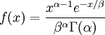$f(x) = \frac{x^{\alpha - 1} e^{-x/\beta}}{\beta^{\alpha} \Gamma(\alpha)}$

Note that that $\Gamma(\alpha)$ in the density function refers to the gamma function (which is distinct from the gamma distribution). The gamma function is easy to calculate when its argument is a positive integer:

$\Gamma(x) = (x-1)!$

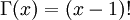
When, however, the argument is an arbitrary positive real number (which is the usual situation for $\alpha$), then computing it gets more complicated. Fortunately, R handles details like this for us!

When the gamma distribution is used to model rate heterogeneity in phylogenetics, its mean is set to 1 because it is being used to model relative rates. In this application, only the shape parameter $\alpha$ is ever specified, and that is because the scale parameter $\beta$ is determined by the constraint that the mean is 1.0.

What is the value of $\beta$ if $\alpha$ is known and the mean must be 1.0?

Creating a Histogram

Let's begin by drawing 1000 random numbers (deviates) from a gamma distribution (shape=0.5, scale=2.0) and creating a histogram. Type the following command into the R console to generate the random deviates and store them in the variable x:

> x = rgamma(1000, shape=0.5, scale=2.0)

The "r" in "rgamma" stands for "random". There is an "r*" command for all the common probability distributions (e.g. rbeta, rbinom, rchisq, rexp, rnorm, runif) and in each case it allows you to draw a sample of values from that distribution (e.g. the beta, binomial, chi-square, exponential, normal and uniform distributions, respectively).

It may appear that nothing has happened, but you can view the 1000 values stored in the variable x by typing x at the prompt.

Creating a basic histogram from these 1000 values is easy:

> hist(x)

Now refine the histogram by telling R that you want there to be 50 bars:

> hist(x, breaks=50)

Now you create a histogram with 40 bars from 10000 deviates from a Gamma(shape=10, scale=0.1) distribution

Create a histogram with 30 bars from 10000 deviates from a gamma distribution in which the mean is 2 and the variance is 1

Plotting the density function

The "d*" commands (e.g. dgamma, dbeta, dexp, dnorm, dunif) can be used to compute the probability density function for a series of values. In this part of the tutorial, you will use the dgamma function to compute the gamma density function for all 501 values in the series 0.0, 0.01, 0.02, ..., 5.0. First, generate the values in the series and store in a variable named x:

x = seq(0.0, 5.0, 0.01)

The seq generates a series of values starting at the first supplied value (0.0 in this case), stopping at the second supplied value (5.0 in this case), with spacing between values in the sequence determined by the third supplied value (0.01 in this case). To see if 501 values were generated, type

length(x)

You can list all the values in x by simply typing x at the console.

R makes it easy to compute a quantity for every number in a list. Here is how to compute the gamma density function value at each value stored in the variable x:

y = dgamma(x, shape=10, scale=0.01)

Before plotting the density function, you should convince yourself that R is computing the density correctly by doing one value yourself by hand. First print out the 100th x value as follows:

x[101]

(Note that indexes begin at 0 in R (as in most programming languages), so the first value is x[0], the second is x[1], and so forth. That's why the 100th value has index 101.) The value displayed should be 1.

Calculate (using the calculator application on your computer) the gamma density for the value 1.0 using $\alpha$=10 and $\beta$ = 0.1

Compare your value to the value computed by R:

y[101]

Now plot the density function as follows:

plot(x,y)

This command says to plot all possible pairs of points, where one value is taken from x and the other from y. There are 501 values in both x and y, so 501 points will be plotted. This plot looks kindof ugly with lots of overlapping points. More reasonable would be to connect the points with a line but not to print all 501 points themselves. You can do this by adding type="l" to your plot command:

plot(x,y,type="l")

The type is specified to be a lower case L character here (L for line). For other plot types, see the online help by typing:

help(plot)