Phylogenetics: R Primer

	EEB 349: Phylogenetics
	This lab represents an introduction to the R computing language, which will be useful for upcoming homework assignments as well as for software written as R extensions (i.e. APE)

What is R?

R is one of two programming languages that we will use this semester (the other being Python). One might make the case that programs like PAUP that are associated with a unique command language also represent programming languages; however, R and Python are different in being general purpose (i.e. not written specifically for phylogenetics).

While R and Python share many similarities, R excels in tasks that involve statistics and creating plots. While a spreadsheet program like Excel can create charts, it is often easier to create the plot you need in R. The purpose of this lab is to introduce you to R by showing you how to make various plots related to probability distributions. This will also enable you to learn about several important probability distributions that serve as prior distributions in Bayesian phylogenetics.

Installing R

Install the R package by going to http://www.r-project.org/ and following the download instructions for your platform.

Plotting the gamma probability density function

As an introduction to R, let's use it to explore the gamma distribution. The gamma distribution has two parameters that govern its shape and scale. Here are some basic facts about gamma distribuitons:

Shape parameter	$\alpha$
Scale parameter	$\beta$
Mean	$\alpha \; \beta$
Variance	$\alpha \; \beta^2$
Density function	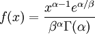$f(x) = \frac{x^{\alpha - 1} e^{\alpha/\beta}}{\beta^{\alpha} \Gamma(\alpha)}$

Note that that $\Gamma(\alpha)$ in the density function refers to the gamma function (which is distinct from the gamma distribution). The gamma function is easy to calculate when its argument is a positive integer:

$\Gamma(x) = (x-1)!$

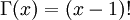
When, however, the argument is an arbitrary positive real number (which is the usual situation for $\alpha$), then computing it gets more complicated. Fortunately, R handles details like this for us!

When the gamma distribution is used to model rate heterogeneity in phylogenetics, its mean is set to 1 because it is being used to model relative rates. In this application, only the shape parameter $\alpha$ is ever specified, and that is because the scale parameter $\beta$ is determined by the constraint that the mean is 1.0.

What is the value of $\beta$ if $\alpha$ is known and the mean must be 1.0?