Phylogenetics: MrBayes Lab

	EEB 349: Phylogenetics
	The goal of this lab exercise is to introduce you to the most important software for conducting Bayesian phylogenetic analyses, MrBayes. You will also learn how to use the program Tracer to analyze MrBayes' output.

Download MrBayes

Download MrBayes from its MrBayes home page. MrBayes will unpack to form a folder containing several example NEXUS data files and the executable file (MrBayes3.1.2 on Mac, mrbayes.exe on Windows).

Download and save the data file

Save the contents of the file algaemb.nex to a file in the MrBayes folder. Important: unless you are a masochist, save the data file in the MrBayes folder so that MrBayes can easily find it!. This is the same 16S data you have used before (algae.nex), but the original file had to be changed to accommodate MrBayes' eccentricities. While MrBayes does a fair job of reading Nexus files, it chokes on certain constructs. The information about what I had to change in order to get it to work is in a comment at the top of the file (this might be helpful in converting other nexus files to work with MrBayes in the future).

Starting MrBayes

Start MrBayes by double-clicking on the executable. When you see the MrBayes > prompt, type the following and then press the Enter key:

exe algaemb.nex

MrBayes should respond with some information, including the encouraging words "Successfully read matrix" and "Reached end of file".

Creating a MRBAYES block

The next step is to set up an MCMC analysis. There are three commands in particular that you will need to know about in order to set up a typical run: lset, prset and mcmc. The command mcmcp is identical to mcmc except that it does not actually start a run. For each of these commands you can obtain online information by typing help followed by the command name: for example, help prset. This may spew more information than will fit on your screen, however.

Create a MRBAYES block in your Nexus data file. MrBayes does not have a built-in editor, so you will need to use your favorite text editor to edit the algaemb.nex data file. Add the following at the bottom of the file to begin creating the MRBAYES block:

begin mrbayes;
end; 

Note that commands in MrBayes are (intentionally) similar to those in PAUP*, but the differences can be frustrating. For instance, lset ? in PAUP* gives you information about the current likelihood settings, but this does not work in MrBayes. Instead, you type help lset. Also, the lset command in MrBayes has many options not present in PAUP*, and vice versa. Get used to typing help followed by the name of a command in MrBayes to see what options are allowed for a particular command.

Specifying the prior on branch lengths

Exponential(10) density function

prset brlenspr=unconstrained:exp(10.0);

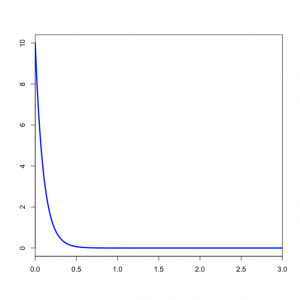
The above command specifies that branch lengths are to be unconstrained (i.e. a molecular clock is not assumed) and the prior distribution to be applied to each branch length is an exponential distribution with mean 1/10. Note that the value you specify for unconstrained:exp is the inverse of the mean.

Specifying the prior on the gamma shape parameter

Exponential(1) density function

prset shapepr=exp(1.0);

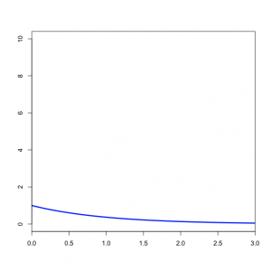
This command specifies an exponential distribution with mean 1.0 for the shape parameter of the gamma distribution we will use to model rate heterogeneity. Note that we have not yet told MrBayes that we wish to assume that substitution rates are variable - we will do that using the lset command below.

Specifying the prior on kappa

Beta(1,1)

kappa density function

prset tratiopr=beta(1.0,1.0);

The command above says to use a Beta(1,1) distribution as the prior for the transition/transversion rate ratio. You may be thinking that it is a little strange to use a Beta distribution for a parameter that ranges from 0 to infinity, and if so you would be right! Allow me to explain as best I can. Recall that the kappa parameter is the ratio $\alpha/\beta$, where $\alpha$ is the rate of transitions and $\beta$ is the rate of transversions. Rather than allowing you to place a prior directly on the ratio $\alpha/\beta$, which ranges from 0 to infinity, MrBayes asks you to instead place a joint (Beta) prior on $\alpha$ and $\beta$. Here, $\alpha$ and $\beta$ act like $p$ and $1-p$ in the familiar coin flipping experiment. The reasoning behind this is esoteric, but is the same as the reasoning behind the (now commonplace) use of Dirichlet priors for the GTR relative rates, which is explained nicely in Zwickl and Holder (2004).

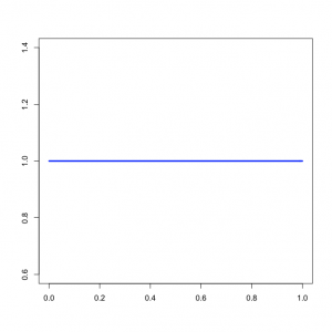
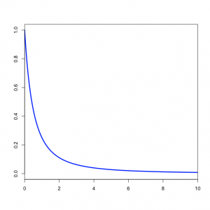
You might wonder what the Beta(1,1) distribution (figure on the left) implies about kappa. It turns out that it is similar (but not identical) to an Exponential(1) distribution (figure on the right).

Specifying a prior on base frequencies

 prset statefreqpr=dirichlet(1.0,1.0,1.0,1.0);

The above command states that a flat dirichlet distribution is to be used for base frequencies. The Dirichlet distribution is like the Beta distribution, except that it is applicable to combinations of parameters. Like the Beta distribution, the distribution is symmetrical if all the parameters of the distribution are equal, and the distribution is flat if all the parameters of the distribution are equal to 1.0. Using the command above specifies a flat Dirichlet prior, which says that any combination of base frequencies will be given equal prior weight. This means that (0.01, 0.99, 0.0, 0.0) is just as probable, a priori, as (0.25, 0.25, 0.25, 0.25). If you wanted base frequencies to not stray much from (0.25, 0.25, 0.25, 0.25), you could specify, say, statefreqpr=dirichlet(10.0,10.0,10.0,10.0) instead.

The lset command

lset nst=2 rates=gamma ngammacat=4;

We are finished setting priors now, so the command above finishes our specification of the model by telling MrBayes that we would like a 2-parameter substitution matrix (i.e. the rate matrix has only two substitution rates, the transition rate and the transversion rate). It also specifies that we would like rates to vary across sites according to a gamma distribution with 4 categories.

Specifying MCMC options

mcmcp ngen=10000 samplefreq=10 printfreq=100 nruns=1 nchains=2 startingtree=random savebrlens=yes;

The command above specifies most of the remaining details of the analysis.

ngen=10000 tells MrBayes that its robots should each take 10,000 steps. You should ordinarily use much larger values for ngen than this (the default is 1 million steps). We're keeping it small here because we do not have a lot of time and the purpose of this lab is to learn how to use MrBayes, not produce a publishable result. samplefreq=10 says to only save parameter values and the tree topology every 10 steps. printfreq=100 says that we would like a progress report every 100 steps.

nruns=1 says to just do one independent run. MrBayes performs two separate analyses by default.

nchains=2 says that we would like to have 1 heated chain running in addition to the cold chain. Ordinarily you would use at least 3 heated chains; again, we're skimping here to keep things fast while you are learning the ropes.

startingtree=random means that we wish to begin from a random starting tree (as opposed to starting with a specific pre-determined tree topology).

Finally, savebrlens=yes tells MrBayes that we would like it to save branch lengths when it saves the sampled tree topologies.

Specifying an outgroup

outgroup Anacystis_nidulans;

This merely affects the display of trees. It says we want trees to be rooted between the taxon Anacystis_nidulans and everything else.

The autoclose command

set autoclose=yes;

This tells MrBayes that we will not want to continue the run beyond the 10,000 generations specified. If you leave this out, MrBayes will ask you whether you wish to continue running the chains after the specified number of generations is finished.

Running MrBayes and interpreting the results

Now save the file and type

exe algaemb.nex

again into MrBayes to reload the data. Then type

mcmc

This command starts the run. While MrBayes runs, it shows one-line progress reports. The first column is the step number. The next two columns show the log-likelihoods of the separate chains that are running, with the cold chain indicated by square brackets rather than parentheses. The last complete column is a prediction of the time remaining until the run completes. The columns consisting of only -- are simply separators, they have no meaning.

• Do you see evidence that the cold chain and heated chain are swapping with each other?
• Could you determine from this output the total number of times the cold chain and heated chain successfully swapped with each other? (The answer is no, ask us if you are puzzled about why.)

When the run has finished, MrBayes will report various statistics about the run, such as the percentage of time it was able to accept proposed changes of various sorts. These percentages should, ideally, all be between about 20% and 40%, but as long as they are not extreme (e.g. 1% or 99%) then things went well.

• What explanation could you offer if the acceptance rate was very low, e.g. 1%?
• What explanation could you offer if the acceptance rate was very high, e.g. 99%?

The section entitled "State exchange information" reports the number of times the cold chain attempted to swap with the heated chain (lower left) and the proportion of time such attempts were successful (upper right). In our case, since there were only 2 chains, the number of attempted swaps should be the same as the number of generations, i.e. 10,000. If you had run 4 chains, each generation a random pair of chains would attempt a swap, so none of the numbers in the lower triangle would be as large as the number of generations specified.

The sump command

MrBayes saves information in several files. Only two of these will concern us today. One of them will be called algaemb.nex.p. This is the file in which the sampled parameter values were saved. This file is saved in tab-delimited format so that it is easy to import into a spreadsheet program such as Excel. We will examine this file graphically in a moment, but first let's get MrBayes to summarize its contents for us.

At the MrBayes prompt, type the command sump. This will generate a crude graph showing the log-likelihood as a function of time. Note that the log-likelihood starts out low on the left (you started from a random tree, remember), then quickly climbs to a constant value.

Below the graph, MrBayes provides the arithmetic mean and harmonic mean of the marginal likelihood. The harmonic mean is used in estimating Bayes factors, which are in turn useful for deciding which among different models fits the data best on average. We will talk about how to use this value in lecture.

The table at the end is quite useful. It shows the posterior mean, median, variance and 95% credible interval for each parameter in your model based on the samples taken during the run. The credible interval shows the range of values of a parameter that account for the middle 95% of its marginal posterior distribution. If the credible interval for kappa is 3.8 to 6.8, then you can say that there is a 95% chance that kappa is between 3.8 and 6.8 given your data (and of course the model). The parameter TL represents the sum of all the branch lengths. Rather than reported every branch length individually, MrBayes just keeps track of their sum.

The sumt command

Now type the command sumt. This will summarize the trees that have been saved in the file algaemb.nex.t.

The output of this command includes a bipartition (=split) table, showing posterior probabilities for every split found in any tree sampled during the run. After the bipartition table is shown a majority-rule consensus tree containing all splits that had posterior probability 0.5 or above.

If you chose to save branch lengths (and we did), MrBayes shows a second tree in which each branch is displayed in such a way that branch lengths are proportional to their posterior mean. MrBayes keeps a running sum of the branch lengths for particular splits it finds in trees as it reads the file algaemb.nex.t. Before displaying this tree, it divides the sum for each split by the total number of times it encountered the split to get a simple average branch length for each split. It then draws the tree so that branch lengths are proportional to these mean branch lengths.

Finally, the last thing the sumt command does is tell you how many tree topologies are in credible sets of various sizes. For example, in my run, it said that the 99% credible set contained 18 trees. What does this tell us? MrBayes orders tree topologies from most frequent to least frequent (where frequency refers to the number of times they appear in algaemb.nex.t). To construct the 99% credible set of trees, it begins by adding the most frequent tree to the set. If that tree accounts for 99% or more of the posterior probability (i.e. at least 99% of all the trees in the algaemb.nex.t file have this topology), then MrBayes would say that the 99% credible set contains 1 tree. If the most frequent tree topology was not that frequent, then MrBayes would add the next most frequent tree topology to the set. If the combined posterior probability of both trees was at least 0.99, it would say that the 99% credible set contains 2 trees. In our case, it had to add the top 18 trees to get the total posterior probability up to 99%.

Type quit (or just q), to quit MrBayes now.

Using Tracer to summarize MCMC results

Instead of using Excel to examine the contents of this file, we will use a program called Tracer designed specifically for this purpose. Tracer can be downloaded free from the Oxford Evolutionary Biology Group web site, which by the way is a good place to find many useful programs for phylogenetic analysis.

Double-click the shortcut for Tracer on your desktop to start the program. Choose File > Import... (or use the key combination Ctrl-I) to choose a parameter sample file to display. Select the algaemb.nex.p in your working folder, then click the Open button to read it.

You should now see 8 rows of values in the table labeled Traces on the left side of the main window. The first row (LnL) is selected by default, and Tracer shows a histogram of log-likelihood values on the right, with summary statistics above the histogram.

A histogram is perhaps not the most useful plot to make with the LnL values. Click the Trace tab to see the kind of plot I termed a history plot in lecture.

Tracer determines the burn-in period using an undocumented algorithm. You may wish to be more conservative than Tracer. Opinions vary about burn-in. Some Bayesians feel it is important to exclude the first few samples because it is obvious that the chains have not reached stationarity at this point. Other Bayesians feel that if you are worried about the effect of the earliest samples, then you definitely have not run your chains long enough!

Click the Estimates tab again at the top, then click the row labeled kappa on the left.

• What is the posterior mean of kappa?
• What is the 95% credible interval for kappa?

Click the row labeled alpha on the left. This is the shape parameter of the gamma distribution governing rates across sites.

• What is the posterior mean of alpha?
• What is the 95% credible interval for alpha?
• Is there rate heterogeneity among sites, or are all sites evolving at nearly the same rate?

Click on the row labeled TL on the left (the Tree Length).

• What is the posterior mean tree length?
• What is the mean edge length? (Hint: divide the tree length by the number of edges, which is 2n-3 if n is the number of taxa.)

Running MrBayes with no data

Why would you want to run MrBayes with no data? Here's a possible reason. You discover by reading the text that results from typing help prset that MrBayes assumes, by default, the following branch length prior: exp(10). What does the 10 mean here? Is this an exponential distribution with mean 10 or is 10 the so-called "hazard" parameter (a common way to parameterize the exponential distribution)? If 10 is correctly interpreted as the hazard parameter, then the mean of the distribution is 1/hazard, or 0.1. Ideally, the documentation of MrBayes should tell you this sort of information, but often such details are left out (and they are left out in this case).

Also, it is not possible to place prior distributions directly on some quantities of interest. For example, while you can specify a flat prior on topologies, it is not possible to place a prior on a particular split you are interested in. This is because the prior distribution of splits is an induced prior; that is, it is determined indirectly by the prior you place on topologies. Running a Bayesian MCMC program without data is a good way to make sure you know what priors you are actually placing on the quantities of interest. Even if you think you know, running dataless provides a good sanity check. If there is no information in the data, the likelihood is 1.0 (and the log-likelihood is thus 0.0) for every parameter combination and tree topology. Running MrBayes without data thus effectively takes the likelihood out of Bayes formula, and the posterior distribution equals the prior distribution. An MCMC analysis thus provides an approximation of the prior. Let's see how this works...

Execute the file blank.nex in MrBayes. Here is what this file looks like (use PAUP*'s editor to create this file):

 #nexus
 begin data;
 dimensions ntax=4 nchar=1;
 format datatype=dna missing=? gap=-;
 matrix
   A ?
   B ?
   C ?
   D ?
   ;
 end;
 
 begin mrbayes;
   prset brlenspr=unconstrained:exp(10.0);
   prset tratiopr=beta(1.0,1.0);
   prset statefreqpr=Dirichlet(1.0,1.0,1.0,1.0);
   prset shapepr=exp(1.0);
   lset nst=2 rates=gamma ngammacat=4;
   mcmcp ngen=1000000 samplefreq=100 printfreq=10000 nruns=1 nchains=1;
 end;

Note that the data matrix is composed of just one character, and that character is composed of only missing data!

Type mcmc to perform the analysis. Because calculation of the likelihood is the most time-consuming part of a Bayesian analysis, this analysis will go quickly because the likelihood takes almost no time to compute in this case.

Checking the shape parameter prior

Import the output file blank.nex.p in Tracer. Look first at the histogram of alpha, the shape parameter of the gamma distribution.

• What is the mean you expected for alpha based on the prset shapepr=exp(1.0) command in the blank.nex file?
• What is the posterior mean actually estimated by MrBayes (and presented by Tracer)?
• An exponential distribution always starts high and approaches zero as you consider higher and higher values. The highest point of the exponential density function is 1/mean. If you look at the approximated density plot (click on the Density tab), does it appear to approach 1/mean at the value alpha=0.0?

Checking the branch length prior

Now look at the histogram of TL, the tree length.

• What is the posterior mean of TL, as reported by Tracer?
• What value did you expect based on the prset brlenspr=unconstrained:exp(10) command?
• Does the approximated posterior distribution of TL appear to be an exponential distribution?

The second and third questions are a bit tricky, so I'll just give you the explanation. Please make sure this explanation makes sense to you, however, and ask us to explain further if it doesn't make sense. We told MrBayes to place an exponential prior with mean 0.1 on each branch. There are 5 branches in a 4-taxon, unrooted tree. Thus, 5 times 0.1 equals 0.5, which should be close to the posterior mean you obtained for TL. That part is fairly straightforward.

The marginal distribution of TL does not look at all like an exponential distribution, despite the fact that TL should be the sum of 5 exponential distributions. The famous Central Limit Theorem in statistics says that if you add together several independent random quantities, the distribution of the sum will approximate a normal distribution. The approximation gets better the more items there are in the sum. Also, it doesn't even matter how the individual random quantities are distributed , their sum will have a normal distribution (or something close to a normal distribution). If you have trouble believing this, play with the Java applet I wrote to demonstrate the Central Limit Theorem.

Other output files produced by MrBayes

That's it for the lab today. You can look at plots of the other parameters if you like. You should also spend some time opening the other output files MrBayes produces in PAUP*'s editor to make sure you understand what information is saved in these files. Note that some of MrBayes' output files are actually Nexus tree files, which you can open in TreeView. For example, algaemb.nex.con contains the consensus tree from the Bayesian analysis, and algaemb.nex.t contains the sampled trees. The file algaemb.nex.trprobs contains all distinct tree topologies, sorted from highest to lowest posterior probability. You may wish to add the suffix .tre to these files so that TreeView recognizes them as tree files (allowing you to open them in TreeView with a double-click).

Literature Cited

- ↑ Zwickl, D., and Holder, M. T. 2004. Model parameterization, prior distributions, and the general time-reversible model in Bayesian phylogenetics. Systematic Biology 53(6):877–888