Phylogenetics: Phycas Lab

|
EEB 349: Phylogenetics |
| The goal of this lab is to introduce you to some of the features of Phycas, which is a Bayesian phylogenetic analysis program that I am co-authoring with Mark Holder (University of Kansas) and David Swofford (Duke University). Phycas is a juvenile compared to MrBayes and Beast, but it nevertheless allows you to do some things that neither of those programs do. We will use Phycas for two of these today: (1) perform MCMC analyses that allow polytomies; and (2) obtain accurate estimates of marginal likelihoods that can be used to compute Bayes Factors. |
Contents
Downloading Phycas
The home page for Phycas is phycas.org (this URL actually points to a section of the EEB department's web site, so you will see the address change to one involving hydrodictyon.eeb.uconn.edu as it loads). In the download section of that web site, you will see links for the Windows version, the Mac version and the PDF manual; however DO NOT DOWNLOAD THESE! I had to fix a few bugs before this lab exercise would work correctly, so I created a new release for you to use today (I will update the main web site in the next week or so):
Installing and starting Phycas in interactive mode
To start using Phycas interactively, simply click the Phycas icon on the dock. This starts a special version of the iTerm program (called iTerm4Phycas) and, after loading the Phycas libraries, presents you with the python prompt (>>>).
We admit that it is somewhat confusing to bundle iTerm with Phycas: for example, all the menu items are iTerm menu items and have nothing to do with Phycas! Phycas is an extension of Python, so you invoke Phycas' capabilities by issuing Python commands at the command prompt, not by using the menus. Due to a glitch in iTerm, you may wish to issue a couple of Command+U commands using your keyboard to eliminate transparency in the background of the iTerm window.
To start using Phycas interactively, open a command prompt window and type python to start python. Now type
from phycas import *
to import everything Phycas can do into Python. You are now ready to begin issuing Phycas-specific Python commands.
Finding help
Most of the time, you will use Phycas in batch mode: that is, you will create a file containing Python code and simply run that file the way you run any Python script (e.g. python myscript.py). It is handy, however, to run Phycas interactively because the online help facility can be consulted as you build up your script.
First, to see what major function Phycas supports, type the following. Note that in all discussions of using Phycas interactively, I will include the Python prompt (>>>), but you should not type the three greater-than symbols:
>>> help()
In the output that follows, you should see some part that looks like this:
The currently implemented Phycas commands are:

like                           randomtree
mcmc                           sim
model                          sump
ps                             sumt
For any of these commands, you can get more information about the command by typing the name of the command followed by a period and the word help. For example,
>>> model.help
produces this output (just the first part of the output is shown:
Help entry for <phycas.Phycas.Model.Model object at 0x746450>:
model
Defines a substitution model.

Available input options:
Attribute                      Explanation
============================== =================================================
type                           Can be 'jc', 'hky' or 'gtr'

update_relrates_separately     If True, GTR relative rates will be individually
                               updated using slice sampling; if False, they will
                               be updated jointly using a Metropolis-Hastings
                               move (generally both faster and better).

relrate_prior                  The joint prior distribution for all six GTR
                               relative rate parameters. Used only if
                               update_relrates_separately is False.

relrate_param_prior            The prior distribution for individual GTR
                               relative rate parameters.  Used only if
                               update_relrates_separately is true.

relrates                       The current values for GTR relative rates. These
                               should be specified in this order: A<->C, A<->G,
                               A<->T, C<->G, C<->T, G<->T.
...
To skip the explanation of each setting and instead see a concise table of the current values for each setting, try this:
>>> model.curr
This produces the following output:
Current model input settings:

Attribute                      Current Value
============================== =================================================
type                           'hky'
update_relrates_separately     True
relrate_prior                  Dirichlet((1.00000, 1.00000, 1.00000, 1.00000,
                               1.00000, 1.00000))
relrate_param_prior            Exponential(1.00000)
relrates                       [1.0, 4.0, 1.0, 1.0, 4.0, 1.0]
fix_relrates                   False
kappa_prior                    Exponential(1.00000)
kappa                          4.0
fix_kappa                      False
num_rates                      1
gamma_shape_prior              Exponential(1.00000)
gamma_shape                    0.5
fix_shape                      False
use_inverse_shape              False
pinvar_model                   False
pinvar_prior                   Beta(1.00000, 1.00000)
pinvar                         0.2
fix_pinvar                     False
update_freqs_separately        True
state_freq_prior               Dirichlet((1.00000, 1.00000, 1.00000, 1.00000))
state_freq_param_prior         Exponential(1.00000)
state_freqs                    [1.0, 1.0, 1.0, 1.0]
fix_freqs                      False
edgelen_hyperprior             InverseGamma(2.10000, 0.90909)
fix_edgelen_hyperparam         False
edgelen_hyperparam             0.05
internal_edgelen_prior         Exponential(2.00000)
external_edgelen_prior         Exponential(2.00000)
edgelen_prior                  None
fix_edgelens                   False
use_flex_model                 False
flex_ncat_move_weight          1
flex_num_spacers               1
flex_phi                       0.25
flex_L                         1.0
flex_lambda                    1.0
flex_prob_param_prior          Exponential(1.00000)
============================== =================================================
Using Phycas to allow polytomies in Bayesian phylogenetic analyses
Simulating data on a polytomous tree
One strength of Phycas is that it allows topology priors that allow for the possibility that there are polytomies in the true tree. Instead of analyzing actual sequence data, you will simulate a data set using Phycas using a polytomous model tree. You will then analyze the data in Phycas under a topology prior that either allows or disallows polytomies to see if the "star tree paradox" is evident. Each person will choose their own pseudorandom number seed, so at the end we should have results from several different simulation replicates for comparison.
The first step is to create a Python script that will simulate the data. Create a new file named sim.py and copy the following text into it:
from phycas import *
setMasterSeed(13579)
sim.taxon_labels = ['A','B','C','D','E','F','G','H','I','J','K','L','M']
sim.tree_source = TreeCollection(newick='((1,(2,3)),(4,5,(6,7)),(8,(9,10)),(11,(12,13)))')
sim.nchar = 10000
sim.file_name = 'simulated.nex'
sim()
This file accomplishes the following:
- imports the Phycas module into Python
- sets the global pseudorandom number seed (please choose your own seed so we don't all end up with identical results)
- specifies the taxon labels
- specifies the tree topology that we wish to use as the model tree (the numbers in this tree description correspond to the labels in the taxon_labels list)
- specifies the number of sites to generate
- specifies the name of the file to generate
- says to "Make it so, number 1" (i.e., actually perform the simulation)
Since we did not specify the model, it will use the default model (use the model.curr command to see all the current settings for the model).
Run this file by (Mac users) dragging it from a finder window onto the Phycas icon in your dock or (Windows users) opening a console window in the folder where sim.py is located and typing python sim.py.
Note to Mac users: you should always quit Phycas completely before dragging a new file onto its icon. To quit it completely, click on the icon to bring it to the forefront, then choose "Quit iTerm" from the iTerm4Phycas menu or press Command-Q using the keyboard.
Performing a standard MCMC analysis
Create a second file named standardmcmc.py and copy the following text into it:
from phycas import *

setMasterSeed(13579)

mcmc.data_source = 'simulated.nex'
mcmc.ncycles = 2000
mcmc.sample_every = 1
mcmc.allow_polytomies = False
mcmc()
This file accomplishes the following:
- the first line imports the Phycas module into Python
- setMasterSeed sets the seed used by the MCMC analysis
- mcmc.data_source specifies the data file name
- mcmc.ncycles specifies the number of update cycles (a cycle in Phycas is analogous to, but quite different than, a generation in MrBayes --- more on this later)
- mcmc.sample_every specifies the number of cycles before the next sample is saved (in this case, a sample is saved after every cycles, which will result in 2000 lines in the parameter file params.p and 2000 lines in the tree file trees.t)
- mcmc.allow_polytomies specifies whether or not polytomies will be allowed (the answer is no here, but we will do a second analysis later that allows them)
- mcmc() says to start the MCMC analysis
While the MCMC analysis is running...
After an initial dump of information about parameters and their priors, Phycas quiets down and only outputs a summary line like the following every 100 cycles:
cycle = 100, lnL = -89198.17244 (20.79998 secs)
The time shown is the elapsed time in seconds. Periodically, Phycas adjusts the efficiency of its slice samplers, and after each such adjustment outputs a summary like the following:
Slice sampler diagnostics:
  mode=0.20992, avgevals=6.730 (edge length hyperparameter)
  mode=0.11629, avgevals=7.850 (edge length hyperparameter)
  mode=3.94956, avgevals=6.620 (trs/trv rate ratio)
  mode=1.08247, avgevals=9.080 (base freq. A)
  mode=1.10869, avgevals=8.770 (base freq. C)
  mode=1.07547, avgevals=8.580 (base freq. G)
  mode=1.09889, avgevals=8.830 (base freq. T)
For each parameter (or hyperparameter) being updated by a slice sampler, the mode and average number of evaluations per update is reported. The mode is simply that value of the parameter associated with the highest posterior density during the time since the slice samplers were last adjusted. This gives you a rough idea of the current location of the parameter. The avgevals value is the average number of times the posterior density needed to be computed in order to obtain a valid new sample of the parameter.
You might have noticed that the base frequencies seem to be out of bounds (all four modes are greater than 1). Base frequency parameters in Phycas are by default left unnormalized unless they are being used in computing the likelihood. This makes it easier for the base frequencies to be independently updated by slice sampling: the slice sampler updating the frequency of A does not have to coordinate with the other three slice samplers to ensure that the sum of the base frequencies is 1.0.
Two of the entries above represent edge length hyperparameters. Rather than placing a prior directly on edge length parameters, Phycas creates two new hyperparameters that represent the prior means of branch lengths. One governs the prior mean of the internal edge lengths, the other governs the prior mean of the external edge lengths. Phycas allows you to override this default behavior if you wish and place a prior directly on either group of edge lengths.
At the end of the run, Phycas tells you how many times the likelihood function was evaluated and how long it took:
283250 likelihood evaluations in 364.22067 seconds
  = 777.68788 likelihood evaluations/sec
Summarizing trees
The sumt command is used to summarize trees and splits. Type the following commands at the Python prompt:
>>> sumt.trees = 'trees.t'
>>> sumt()
The output includes a standard table of splits found:
split       pattern freq.      prob.     weight    s0    sk     k
    1 -*-----------  2000    1.00000    0.00109     1  2000     1
    2 -------*-----  2000    1.00000    0.05262     1  2000     1
    3 -************  2000    1.00000    0.05490     1  2000     1
    4 -----------*-  2000    1.00000    0.04698     1  2000     1
    5 ----*--------  2000    1.00000    0.09359     1  2000     1
    ...
The only unusual features here are s0, sk and k. The value k represents the number of sojourns, where a sojourn is a stretch of consecutive samples in which the split appears. All the splits shown in the snippet above were present in every sample, so their single sojourns all started with the first sample and ended with the last sample. s0 and sk record the beginning of the first sojourn and the end of the last sojourn, respectively. For splits that have posterior probabilities less than 1, the number of sojourns gives you some information about how often the MCMC robots returned to a split once they left it. In general, more sojourns are better than only 1 sojourn.
A similar table summarizes results for entire tree topologies:
topology freq.         TL    s0    sk     k      prob.       cum.
       1   780    2.36431    53  1984    39    0.39000    0.39000
       2   375    2.35733    35  2000    29    0.18750    0.57750
       3   311    2.36594    93  1924    23    0.15550    0.73300
       4   173    2.36237   150  1859    16    0.08650    0.81950
       5    92    2.36926   146  1882    10    0.04600    0.86550
       6    88    2.36453   543  1741     6    0.04400    0.90950
       7    74    2.36172    31  1839    14    0.03700    0.94650
       8    38    2.37042   283  1908     7    0.01900    0.96550
Here, freq. is the number of samples in which a tree topology appears, TL is the posterior mean tree length, prob. is the posterior probability of the tree (the frequency divided by the total number of samples), and cum. is the cumulative posterior probability of the tree.
- How many tree topologies are in the 95% credible set for your run? The answer is 8 for the run summarized above because all eight trees visited during the run must be included in order to make the cumulative posterior probability greater than 0.95. Likewise, 6 trees are in the 90% credible set and only 2 trees are in the 50% credible set.
Several files were created by the sumt command. sumt_splits.pdf comprises two plots. The first page plots the most important splits through time, allowing you to see whether the run achieved convergence with respect to the topology. If there are a lot of lines crossing, especially toward the end of the run, then things did not go well. The second page contains the Split Sojourns plot. This plot shows the sojourns of the most important splits. As you can see, some splits were present from start to finish, whereas many splits only existed for a short time at the start of the run. If things went well, then the intermediate splits should show a pattern of coming and going often.
The sumt_trees.pdf file shows the majority rule consensus tree on page 1 followed by the trees comprising the 95% credible set, each on a separate page thereafter. The title of each page shows the frequency of the tree shown on that page.
- Looking at the majority rule tree, do you see the polytomy present in the model tree that you used for simulating the data? The four groups that should form the polytomy are (A,B,C), (D,E,F,G), (H, I, J), and (K, L, M).
- If any two of these four groups are joined together in the majority rule tree, what is the posterior probability of that group?
The sumt_trees.tre file is a NEXUS tree file containing the tree descriptions of the trees in the 95% credible set (i.e. the same trees that are shown graphically in the sumt_trees.pdf file.
Performing a polytomy-friendly MCMC analysis
Create a file named polymcmc.py and copy the following text into it:
from phycas import *

setMasterSeed(13579)

mcmc.data_source = 'simulated.nex'
mcmc.ncycles = 2000
mcmc.sample_every = 1
mcmc.allow_polytomies = True
mcmc.out.log = 'polytomy.txt'
mcmc.out.trees = 'polytomy.t'
mcmc.out.params = 'polytomy.p'
mcmc()
The main differences between this analysis and the previous one are that:
- mcmc.allow_polytomies is set to True this time
- the three output files have been given names so that we don't overwrite the files from the standard analysis
Please make up your own seed again for this run so we get a variety of answers
While the MCMC analysis is running...
At the beginning of this run, you should see the following description of the topology prior, including the distribution of prior probability across resolution classes, where a resolution class is indexed by the number of internal nodes (class 1 has only one internal node, and thus corresponds to the "star tree"):
Topology prior:
  Prior type: polytomy prior
  Prior strength (C): 2.0
  Prior probability for each resolution class:
  Note: 0.00000000 does *not* mean that the prior is zero! It simply
        indicates that the prior is less than 0.000000005

      internal nodes    prior probability
      --------------    -----------------
                   1           0.00000000
                   2           0.00000180
                   3           0.00016101
                   4           0.00340514
                   5           0.02810290
                   6           0.11288241
                   7           0.24606615
                   8           0.30493415
                   9           0.21384408
                  10           0.07878466
                  11           0.01181770
Note that most of the prior probability mass is on tree topologies that are not fully resolved. Fully-resolved tree topologies have 11 internal nodes (ntaxa-2, where ntaxa=13 in this case), and these trees as a group have only 1% of the prior probability. This means that if you ran an MCMC sampler without data, about 99% of the trees sampled would have at least 1 polytomy. The stength of the prior is determined by the setting mcmc.topo_prior_C, which we did not explicitly set in this case, so it took on the default value of 2.0. If you set topo_prior_C to be larger than 2, unresolved trees would get even more of the prior probability. Setting topo_prior_C to be 1.0 yields the flat prior: every tree topology has equal prior weight regardless of how resolved it is. Note that the flat prior still fairly heavily favors unresolved trees because there are many more unresolved trees than there are resolved ones (out of 188,666,182,784 total tree topologies for 13 taxa, 13,749,310,575 (7%) are fully resolved and 174,916,872,209 (93%) have other levels of resolution.
If you ever want or need to compute the number of tree topologies, here's how to do it in Phycas (which uses the method described in chapter 3 entitled "How many trees are there?" of Joe Felsenstein's book[1]):
>>> tpcalc = Likelihood.TopoPriorCalculator()  # create a topology prior calculator
>>> tpcalc.chooseUnrooted()       # call chooseRooted() if you want numbers for rooted trees instead
>>> tpcalc.getLnTotalCount(13)    # get log of total number of trees for 13 taxa
25.963245061729079
>>> math.exp(25.963245061729079)  # exponentiate to get actual number (may need to "import math" first)
188666182784.00009
>>> tpcalc.getLnCount(13,11)      # get log of number of trees for trees with 13 taxa and 11 internal nodes
23.34425451980194
>>> math.exp(23.34425451980194)
13749310574.999998
The slight deviations you see are normal (the result of computers having only a finite number of bits of memory with which to store numbers with an infinite number of decimal places). Just round to the nearest whole number after exponentiating. Note that for many taxa, the number of tree topologies will be too large to obtain - you will receive a "OverflowError: math range error" when you try to exponentiate the log of the count; you will have to settle for having the log of the number in these cases.
Summarizing trees
Use the sumt command again to summarize trees and splits. Type the following commands at the Python prompt:
>>> sumt.trees = 'polytomy.t'
>>> sumt()
The sumt_trees1.pdf file shows the majority rule consensus tree on page 1. Note that Phycas appended the number 1 to the end of the file name because it found a file by the name sumt_trees.pdf already present (from your previous run).
- Looking at the majority rule tree, do you see the polytomy present in the model tree that you used for simulating the data?
In this experiment, we simulated a data set containing a true polytomy. Not surprisingly, when polytomous trees were favored by the tree topology prior, the analysis produced a majority rule summary tree containing that polytomy. One criticism that is always possible with Bayesian analyses is that the prior was too informative and unduly influenced the result.
- What modification of this experiment could you make to counter the potential criticism that the polytomy prior was so strong that it swamped out the information in the likelihood in this case?
Using Phycas to estimate marginal likelihoods accurately
The Bayes factor (BF) is commonly used to decide which of two models is better. The BF is the ratio of the marginal likelihoods of the models in question, so to compute the BF one needs to estimate the marginal likelihoods of the competing models (although methods exist for computing the BF directly in special cases). The harmonic mean estimator is the most commonly used means for obtaining estimates of marginal likelihoods in phylogenetics. MrBayes reports (in its sump output) the log of the harmonic mean of the likelihood over samples taken during an MCMC analysis. The harmonic mean of the likelihood is indeed an estimate of the marginal likelihood, and has the desirable property of being free (it is automatically available after an MCMC analysis - no extra work is required). Unfortunately, it is not a very good estimate of the marginal likelihood, and is quite biased in favor of the more complex model.
Phycas can obtain a better estimate of the marginal likelihood for the models it implements (which includes all the standard models, from JC to GTR+I+G), but doing so requires a special MCMC analysis that cannot be used for anything else (no such thing as a free lunch, remember?). Phycas actually computes the marginal likelihood using two different methods: path sampling (also known as thermodynamic integration) and steppingstone sampling. Path sampling was introduced into phylogenetics by Lartillot and Phillippe (2006)[2]. Steppingstone sampling is a new method that is described in a paper co-authored by me (Paul Lewis) that is currently in review. In this part of the lab, we will compute the marginal likelihood three ways (harmonic mean, path sampling, steppingstone sampling) and compare the results. To keep this within a manageable time frame, we will anaylyze a very small data set (the green5.nex data set you used for homework 8), which lets us get away with short MCMC runs. You should not use the ncycles specified in this lab as a recommendation for analyses of larger datasets!
Download and save the data set
Obtain the data from green5.nex and save it as a file named green5.nex in a folder of your choice.
Create your Phycas Python scripts
Now create a file named hm.py in the same directory with this content (except change the seed):
from phycas import *
setMasterSeed(13579)
mcmc.data_source = 'green5.nex'
mcmc.ncycles = 21000
mcmc.sample_every = 10
mcmc.out.log = 'hm.txt'
mcmc.out.params = 'hm.p'
mcmc.out.trees = 'hm.t'
mcmc()
sump.file = 'hm.p'
sump.out.log = 'hm_sump.txt'
sump.burnin = 101
sump()
This script will run a traditional MCMC analysis and summarize the params file. This will provide the harmonic mean estimator of the marginal likelihood.
Create a second python script named ps.py with the following content (except use your own seed):
from phycas import *
setMasterSeed(13579)
mcmc.data_source = 'green5.nex'
mcmc.ncycles = 1000
mcmc.sample_every = 10
mcmc.out.log = 'ps.txt'
mcmc.out.params = 'ps.p'
mcmc.out.trees = 'ps.t'
ps.nbetavals = 21
ps()
sump.file = 'ps.p'
sump.out.log = 'ps_sump.txt'
sump()
This script will run a special MCMC analysis (invoked by the ps command rather than the mcmc command), and afterward the sump command will compute the steppingstone and path sampling estimators of the marginal likelihood. What's special about this MCMC analysis? It is special because the MCMC sampler is not exploring the posterior distribution! It is instead exploring something called the power posterior:
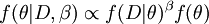
The power posterior,  , differs from the posterior in that the likelihood,
  , is raised to the power
  , where ranges from 0.0 to 1.0. starts at the value 1.0, but is lowered to 0.0 during the course of the run (the setting nbetavals determines the total number of values used). Thus, when the analysis begins, the MCMC sampler is exploring the posterior (beta = 1.0), whereas at the end of the run, it is exploring the prior (beta = 0.0). Both path sampling and steppingstone sampling use samples from this exploration of power posteriors to more accurately estimate the marginal likelihood.
Note that the number of cycles specified in ps.py is much smaller than the number specified in hm.py. When performing a path sampling analysis, the value of ncycles determines the number of cycles used for each value of \beta. Thus, 1000 cycles times 21 beta values equals 21000 cycles total, which is comparable to the amount of computational effort put into the harmonic mean estimation.
Run the scripts
Execute the two python scripts hm.py and ps.py. If you have a dual-core machine, you can save time by starting both of them in different terminal windows and letting them run simultanously. When they are finished, look at the files hm_sump.txt and ps_sump.txt and answer the following questions:
- What is the log of the marginal likelihood using the harmonic mean estimator?
- What is the log of the marginal likelihood using the path sampling estimator?
- What is the log of the marginal likelihood using the steppingstone sampling estimator?
- Are two of these estimates more similar to each other than the third?
- If so, which one is different?
- How is it different? Is it larger or smaller than the other two?